This article is a summary of the StatQuest video made by Josh Starmer. Click here to see the video explained by Josh Starmer.
Introduction In statistics, Machine Learning and other Data Science fields, we optimize a lot of stuff. For example in linear regresion, we optimize the Intercept and Slope, or when we use Logistic Regression we optimize the squiggle. Moreover, in t-SNE we optimize clusters. The interesting thing is that gradient descent can optimize all these things and much more. A good example is the Sum of the Squared Residuals in Regression: in Machine Learning lingo this is a type of Loss Function. The Residual is the difference between the Observed Value and the Predicted Value.

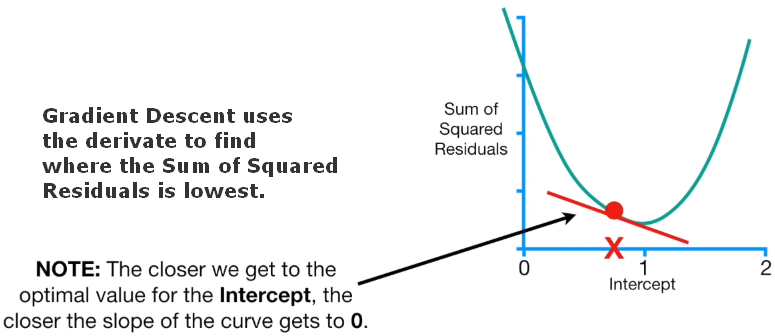
The figure above shows on the y-axis the sum of the squared residuals and the x-axis different value for the intercept. The firt point on the y-axis represent the sum of the squared residuals when the intercept is equal to zero. We continue to plot point on the graph based on different value of the intercept. The lowest poin in the graph has the lowest sum of the squared residuals. Gradient descent identifies the optimal value by taking big steps when we are far away to the optimal sum of the squared residual, and start to make many steps when it is close to the best solution. Than we can calculate the derivate d of each point of the function created by the points. In other words, we are taking the derivative of the Loss Function.

Gradient Descent uses derivative in order to find where the Sum of the Squared Residuals is lowest. The closer we get to the optimal value for the intercept, the closer the slope of the curve gets to zero.
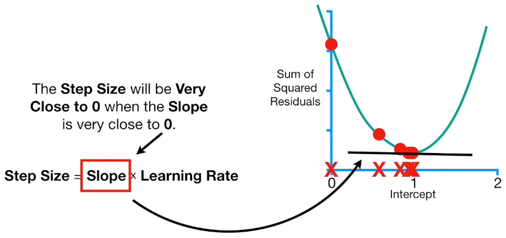
HOW DOES GRADIENT DESCENT KNOW TO STOP TAKING STEPS? Gradient Descent stops when the step size is very close to zero, and the step size is very close to zero qhen the slop size is close to zero.

In practice, the Minimum Step Size is equal to 0.001 or smaller. Moreover, Gradient Descent includes a limit on the number of steps it will take before giving up. In practice, the Maximum Number of Steps is equal to 1000 or greater.
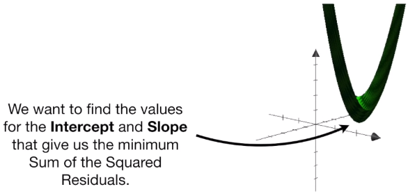
We can also estimate the intercept and the slope simultaneously. We use the Sum of the Squared Residuals as the Loss Function, and we can represent a 3D graph of the Loss Function for different values of intercept and the slope. We want to find the values for the intercept and slope that give us the minumum Sum of the Squared Residuals.

So, just like before, we need to take the derivative of the function represented by the graph above for both intercept and slope. When we have two or more derivatives of the same function (in this case the derivative or both intercept and slope) we call this a GRADIENT. We will use this GRADIANT to DESCENT to lowest point in the Loss Function, which, in this case, is the Sum of the Squared Residuals.
There are tons of other Loss Functions than the Sum of the Squared Residuals, and these Loss Functions work with other types of data. Regardless of which Loss Function is used, Gradient Descent works the same way.
Summarizing: 1 - Take the derivative of the Loss Function for each parameter in it. In ML lingo, take the Gradient of the Loss Function. 2 - Pick random values for the parameters. 3 - Plug the paramenter values into the derivatives (Gradient). 4 - Calculate the Step Sizes: Step Size = Slope * Learning Rate. 5 - Calculate the New Parameters (e.g. intercept): NewParameter = Old Parameter - Step Size. 6 - Go back to step 3 and repeat untill Step Size is very small, or when the Maximum Number of Steps is reached.
Learning rate, used in the calculation of the Steo Size is a hyper-parameter that controls how much we are adjusting the weights with respect of the Loss Function. The lower the values, the slower we travel along the downward slope. This make sure that we do not miss any local minima. Moreover, the learning rate affects how quickly our model can coverge to a local minina (aka arrive at the best accuracy).
One last thing is that when we have millions of data points, the process take a long time. There is a thing called Stochastic Gradient Descent that uses a randomly selected subset of the data at every step rather than the full data. This reduces the time spent calculating the derivatives of the Loss Function.