Text Mining Clustering Tweets

We can use Unsupervised Classification (clustering) to learn more about text that we have to analyze. More specifically, we use Hierarchical clustering to cluster our text into groups that are the propensity to occur together. In this example, text are some tweet about Catalan Independence Referendum.

First step is to convert our tweets into a corpus, remove punctuation, transform everything into lowercase, remove numbers, and stop words. Then, we have to stamming the document, and finally we have a corpus of terms. with out sparse terms.

library(tm)

corpus <- Corpus(VectorSource(d$text))
corpus <- tm_map(corpus, removePunctuation)
corpus <- tm_map(corpus, content_transformer(tolower))
corpus <- tm_map(corpus, removeNumbers)
corpus <- tm_map(corpus, stripWhitespace)
corpus <- tm_map(corpus, removeWords, stopwords('english'))
corpus <- tm_map(corpus, stemDocument)

# Create term document matrix
tdm <- TermDocumentMatrix(corpus,control = list(minWordLength=c(1,Inf)))

t <- removeSparseTerms(tdm, sparse=0.90) # remove words not appear 90% of the time

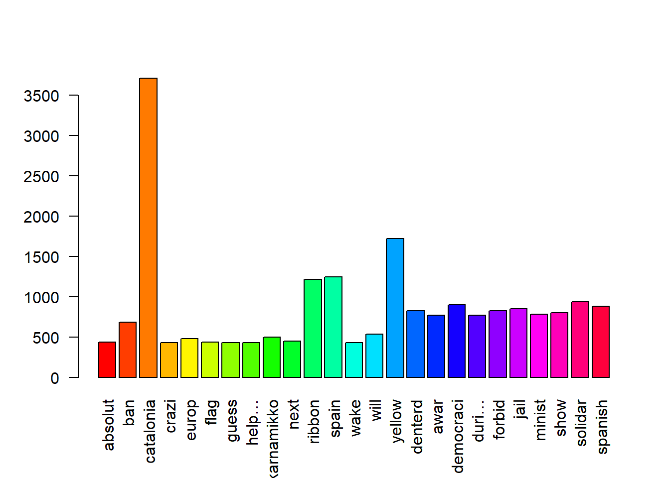
Next step is to create a matrix of word frequency, and we can plot the words that occur more than 200 times, as shown in the graph below.

m <- as.matrix(t) # create a matrix of word frequencies

# Plot frequent terms
freq <- rowSums(m)
freq <- subset(freq, freq>=200)

barplot(freq, las=2, col = rainbow(25))

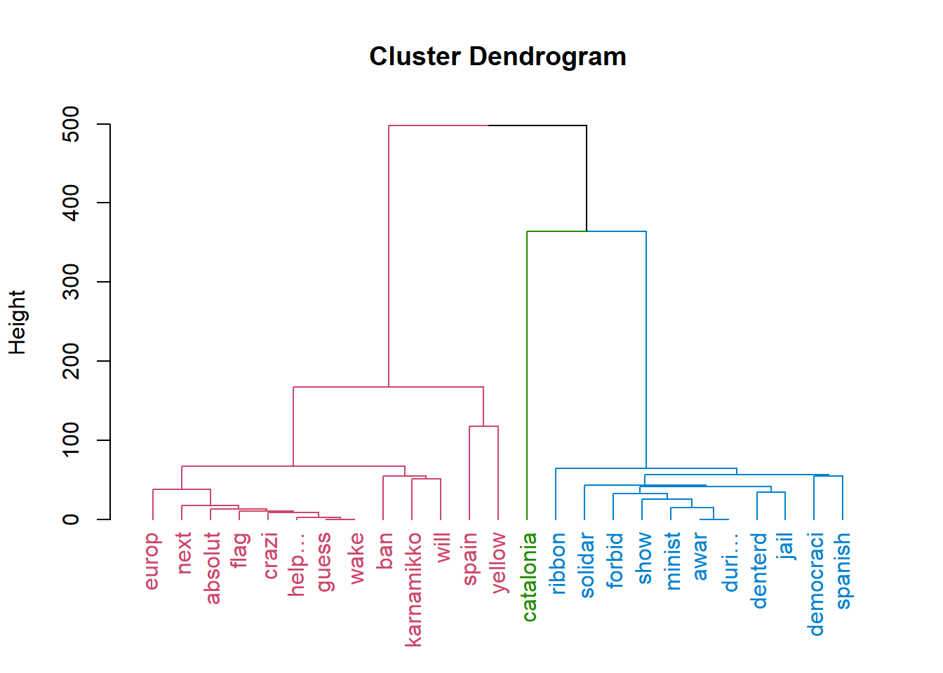
Obviously, catalonia is the most common term, but we have also other interesting high frequency words, such as solidar. Now, we can use Hierarchical clustering of the words using Dendrogram.

# Hierarchical word tweet clustering using dendrogram 

distance <- dist(scale(m)) # distance between different terms

# print(distance, digits = 2)

hc <- hclust(distance, method = "ward.D") # use ward.D for heirarchial clustering
# plot(hc, hang=-1)
# rect.hclust(hc, k=12)

library(dendextend) # color dendrogram

dend <- hc
dend <- color_branches(dend, k = 3)
dend <- color_labels(dend, k = 3)

# Represent the different  clusters with different colors
plot(dend, main = 'Cluster Dendrogram', ylab = 'Height')

From the graph above, we can see that to different cluster has been assigned a different color. To learn more about Hierarchical clustering and Dendrogram, look at this post.