Extract the Main Topics from Books

Topic modeling is the process of identifying topics in a set of documents. This can be useful for search engines, customer service automation, and any other instance where knowing the topics of documents is important. There are multiple methods of going about doing this. The most commonly used is Latent Dirichlet Allocation. The LDA builds a topic per document model and words per topic model, modeled as Dirichlet distributions. For an introduction to Topic Model and LDA please check out this link.

We use the LDA algorithm to correctly distinguish between four groups presented in four different books:
Twenty Thousand Leagues Under the Sea
The War of the World
Pride and Prejudice
Wuthering Heights

All these books can be obtained using the R library gutenbergr which is able to search and download public domain text, as explained in the code below.

library(gutenbergr)
library(tidytext)
library(stringr)
library(topicmodels)
library(dplyr)
library(tidyr)

titles <- c("Twenty Thousand Leagues under the Sea", "The War of the Worlds",
            "Pride and Prejudice", "Wuthering Heights")

books <- gutenberg_works(title %in% titles) %>%
         gutenberg_download(meta_fields = "title") # download the metafiles associated to the titles

Now that we downloaded the boooks we can read them in different chapters.

# Different chapters
by_chapter = books %>%
  group_by(title) %>%
  mutate(chapter = cumsum(str_detect(text, regex("^chapter ", ignore_case = TRUE)))) %>% # ignore the word chapter
  ungroup() %>%
  filter(chapter > 0) %>%
  unite(document, title, chapter) # merge documents by chapter

# Use unnest_tokens() to separate chapters into words, then remove stop_words and split chapters into words
by_chapter_word = by_chapter %>%
  unnest_tokens(word, text)

# Find document-word counts per chapter
word_counts = by_chapter_word %>%
  anti_join(stop_words) %>%
  count(document, word, sort = TRUE) %>%
  ungroup()

# Create a Document Term Matrix(dtm) of word count
chapters_dtm <- word_counts %>%
  cast_dtm(document, word, n)

Now, we are ready to implement the LDA algorithm, and we use K=4 in order to find the four most important topics. From the chapters_dtm above we can see that we are dealing with 168 documents and 17373 terms with a sparcity of 97%.

# We use k=4 as we have 4 books thus 4 distinct themes
chapters_lda <- LDA(chapters_dtm, k = 4, control = list(seed = 1234))

# Examine per-topic-per-word probabilities.
chapter_topics <- tidy(chapters_lda, matrix = "beta")

# Find top 10 terms for each topic
top_terms <- chapter_topics %>%
  group_by(topic) %>%
  top_n(10, beta) %>%
  ungroup() %>%
  arrange(topic, -beta)

At this point, having the top 10 terms per topic we can plot them.

library(ggplot2)
top_terms %>%
  mutate(term = reorder(term, beta)) %>%
  ggplot(aes(term, beta, fill = factor(topic))) +
  geom_col(show.legend = FALSE) +
  facet_wrap(~ topic, scales = "free") +
  coord_flip()

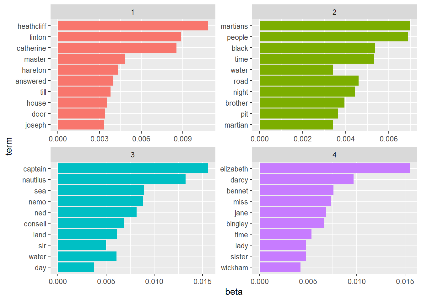
As we can see from the figure above, the Topic 3 contains lots of words related to the book Twenty Thousand Leagues Under the Sea. We can conclude the same for Topic 4 which contains words strongly related to the book Pride and Prejudice. The Topic 2 has words related to the book The War of the World. Finally, the Topic 1 is strongly related to the book Wuthering Heights.

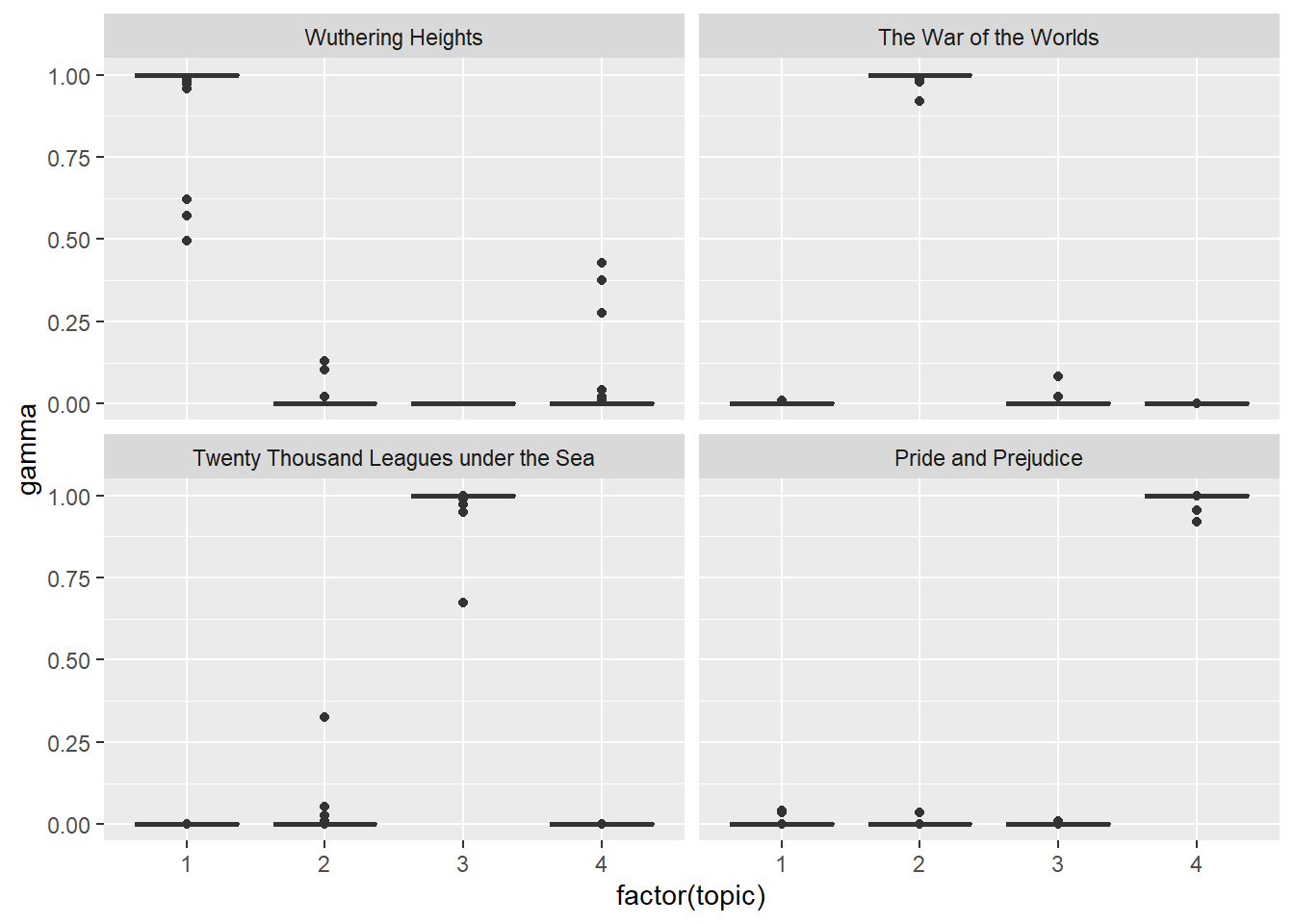
This result tells us that LDA was able to find four distinct topics that reflect the character of the books examined. In order to have a better understanding of the reliability of the LDA we can calculate the association (gamma) of the topic with each document.

# Which topics are associated with each document
chapters_gamma = tidy(chapters_lda, matrix = "gamma")

chapters_gamma = chapters_gamma %>%
  separate(document, c("title", "chapter"), sep = "_", convert = TRUE)

chapters_gamma %>%
  mutate(title = reorder(title, gamma * topic)) %>%
  ggplot(aes(factor(topic), gamma)) +
  geom_boxplot() +
  facet_wrap(~ title)

This assessment assures us that the four books were uniquely identified as a single topic. In fact, all the four books (and their related chapters) are uniquely identified by a single and distinct topic,as we can see from the figure above.