Support Vector Machine SVM is a linear classifier. We can consider SVM for linearly separable binary sets. The goal is to design a hyperplane (is a subspace whose dimension is one less than that of its ambient space. If a space is 3-dimensional then its hyperplanes are the 2-dimensional planes). The hyperplane classifies all the training vectors in two classes. We can have many possible hyperplanes that are able to classify correctly all the elements in the feature set, but the best choice will be the hyperplane that leaves the Maximum Margin from both classes. With Margins we mean the distance between the hyperplane and the closest elements from the hyperplane.
data(iris)
summary(iris)
Sepal.Length Sepal.Width Petal.Length Petal.Width
Min. :4.300 Min. :2.000 Min. :1.000 Min. :0.100
1st Qu.:5.100 1st Qu.:2.800 1st Qu.:1.600 1st Qu.:0.300
Median :5.800 Median :3.000 Median :4.350 Median :1.300
Mean :5.843 Mean :3.057 Mean :3.758 Mean :1.199
3rd Qu.:6.400 3rd Qu.:3.300 3rd Qu.:5.100 3rd Qu.:1.800
Max. :7.900 Max. :4.400 Max. :6.900 Max. :2.500
Species
setosa :50
versicolor:50
virginica :50
head(iris) Sepal.Length Sepal.Width Petal.Length Petal.Width Species
1 5.1 3.5 1.4 0.2 setosa
2 4.9 3.0 1.4 0.2 setosa
3 4.7 3.2 1.3 0.2 setosa
4 4.6 3.1 1.5 0.2 setosa
5 5.0 3.6 1.4 0.2 setosa
6 5.4 3.9 1.7 0.4 setosa# library(ggplot2)
# qplot(Petal.Length, Petal.Width, data=iris, color = Species)We are using the iris dataset with 4 numerical variables and 1 factor which has 3 levels as described above. We can also see that the numerical variables have different ranges, it is a good pratice to normalize the data. We create classification machine learning model that help us to predict the correct species. From the graph above, we can see there is a separation based on the Species, for example setosa species is very far from the other two groups, and between versicolor and virginica there is a small overlap.
With Support Vector Machine SVM we are looking for optimal separating hyperplane between two classes. And to do that SMV maximize the margin around the hyperplane. The point that lie on the boundary ar called Support Vectors, and the middle line is the Seprarating Hyperplane. In situatins where we are not able to obtain a linear separator, the data are projected into a higher dimentional space, so that, data points, can become linearly separable. In this case, we use the the Kernel Trick, using the Gaussian Radial Basis Function.
library(e1071)
mymodel <- svm(Species~., data=iris)
summary(mymodel)
Call:
svm(formula = Species ~ ., data = iris)


Parameters:
   SVM-Type:  C-classification
 SVM-Kernel:  radial
       cost:  1
      gamma:  0.25

Number of Support Vectors:  51

 ( 8 22 21 )


Number of Classes:  3

Levels:
 setosa versicolor virginica
# Plot two-dimensional projection of the data with highlighting classes and support vectors
# The Species classes are shown in different shadings
plot(mymodel, data=iris,
Petal.Width~Petal.Length,
slice = list(Sepal.Width=3, Sepal.Length=4)) # specify a list of named values for the dimensions held constant
# Confusion Matrix and Missclassification Error
pred <- predict(mymodel, iris)
tab <- table(Predicted = pred, Actual = iris$Species)
tab
Actual
Predicted setosa versicolor virginica
setosa 50 0 0
versicolor 0 48 2
virginica 0 2 48# Missclassification Rate
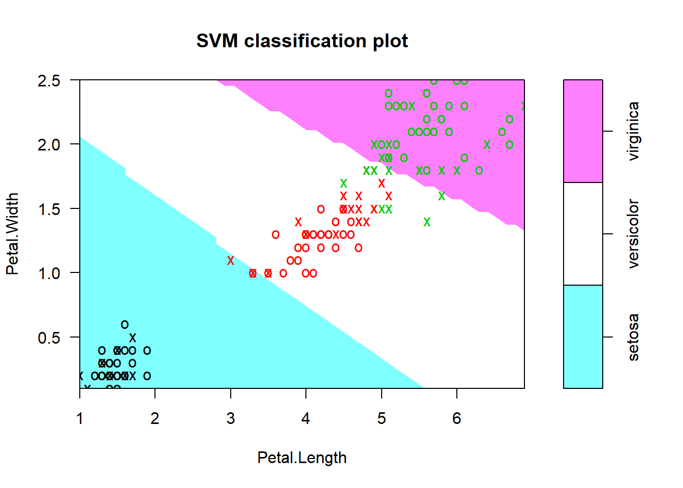
1-sum(diag(tab))/sum(tab)[1] 0.02666667As we can see from the result above, we use Gaussian Radial Basis Function, cost is the constaint violation. The two-dimensional plot above, is a projection of the data with highlighting classes and support vectors. The Species classes are shown in different shadings. Inside the blue class setosa we have 8 points depicted with a cross, and these are the suppor vectors for setosa. Similarly, we have points depicted with red cross points for versicolor, and green cross points for virginica.
From the Confusion Matrix above, we have only 2 observation missclassified for versicolor, and 2 observation missclassified for virginica. We have also a missclassification rate, of 2.6%. If we try to use SVM with a linear kernel (not shown here), instead of a SVM with a radial kernel, the missclassification rate is a bit higher.
mymodel <- svm(Species~., data=iris,
               kernel = "polynomial")

plot(mymodel, data=iris,
     Petal.Width~Petal.Length,
     slice = list(Sepal.Width=3, Sepal.Length=4))
pred <- predict(mymodel, iris)
tab <- table(Predicted = pred, Actual = iris$Species)

1-sum(diag(tab))/sum(tab)
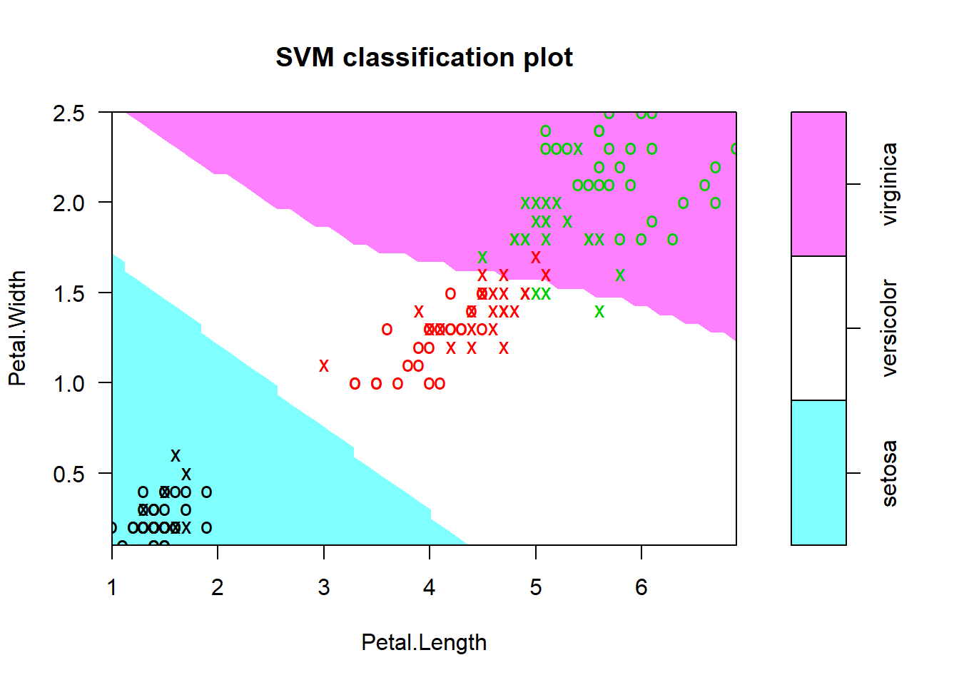
[1] 0.04666667If we also try to use a SVM with a polynomial kernel, as we can see from the graph above, the missclassification rate is increased to 4.6%.
We can try to tune the model in order to have better classification rate. Tune is also called hyperparameter optimization, and it helps to select the best model.
# Tuning
set.seed(123)

tmodel <- tune(svm, Species~., data=iris,
               ranges = list(epsilon = seq(0,1,0.1), # sequence from 0 to 1 with an icrement of 0.1
              cost = 2^(2:7)))                       # cost captures the cost of constant violatio
                                                     # if cost is too high, we have penalty for non-separable points, and the model store too many support vectors

plot(tmodel)
We use epsilon and cost as tune paramentrs. The cost parameter captures the cost of constant violatio. If cost is too high, we have penalty for non-separable points, and as a consequence we have a model that store too many support vectors, leading to overfitting. On the contrary, if cost is too small, we may end up with underfitting.
The value of epsilon defines a margin of tolerance where no penalty is given to errors. In fact, in SVM we can have hard or soft margins, where soft allow observations inside the margins. Soft margin is used when two classes are not linearly separable.
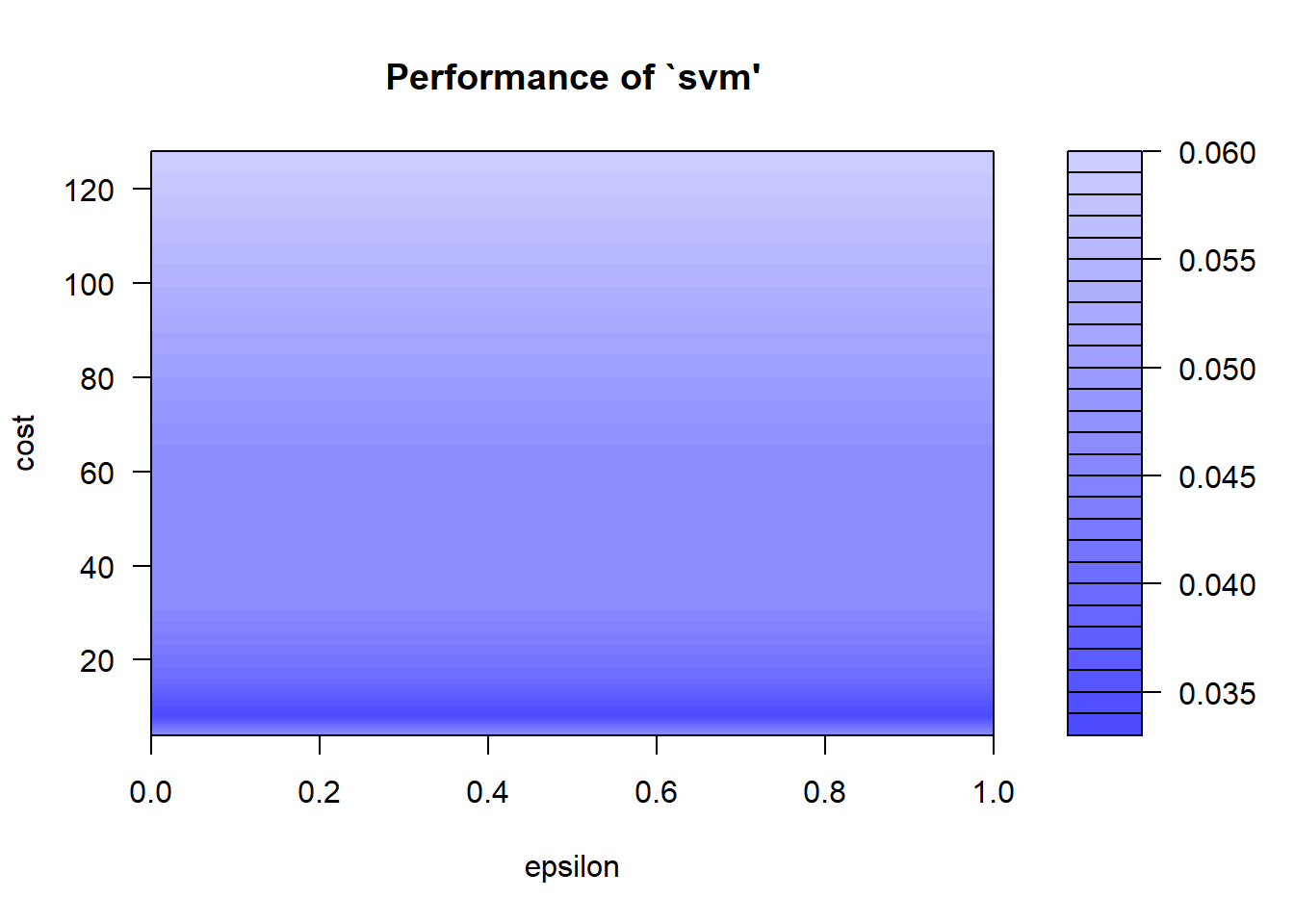
the plot here above gives us the performance evaluation of SMV for the epsilon and cost parameters. Darker regions means better results, and so lower misclassification error. By interpreting this graph we can choose the best model parameters.
mymodel <- tmodel$best.model
summary(mymodel)
Call:
best.tune(method = svm, train.x = Species ~ ., data = iris, ranges = list(epsilon = seq(0,
    1, 0.1), cost = 2^(2:7)))


Parameters:
   SVM-Type:  C-classification
 SVM-Kernel:  radial
       cost:  8
      gamma:  0.25

Number of Support Vectors:  35

 ( 6 15 14 )


Number of Classes:  3

Levels:
 setosa versicolor virginica
plot(mymodel, data=iris,
Petal.Width~Petal.Length,
slice = list(Sepal.Width=3, Sepal.Length=4))
pred <- predict(mymodel, iris)
tab <- table(Predicted = pred, Actual = iris$Species)

1-sum(diag(tab))/sum(tab)
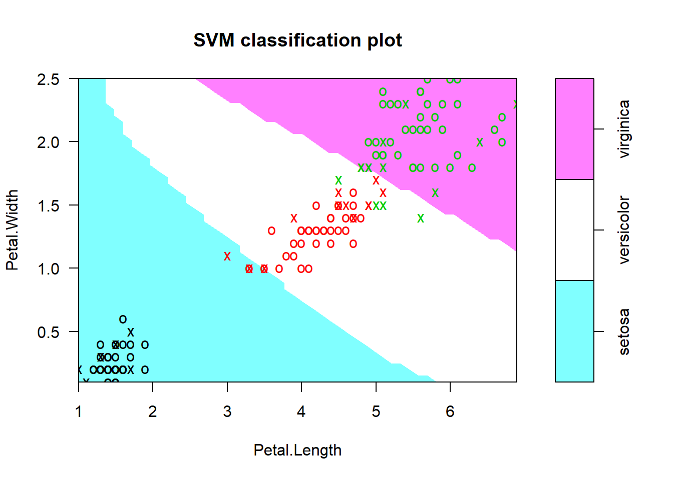
[1] 0.01333333Fomr the summary above, now we have 35 support vectors: 6 for setosa, 15 for versicolor, and 14 for virginica. The graph here above expain the result obtained with the best model. Looking at the confusion matrix and missclassification error, we can see that only 2 observations are missclassified and the missclassification error is 1.3% which is significant less from what the got earlier.