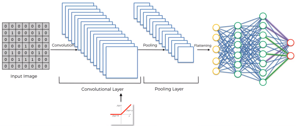
Convolutional neural network CNN is a Supervised Deep Learning used for Computer Vision. The process of Convolutional Neural Networks can be devided in five steps: Convolution, Max Pooling, Flattening, Full Connection.
STEP 1 - Convolution At the bases of Convolution there is a filter also called Feature Detector or Kernel. We basically multiply the portion of the image by the filter and we check the matching how many 1s have in common.
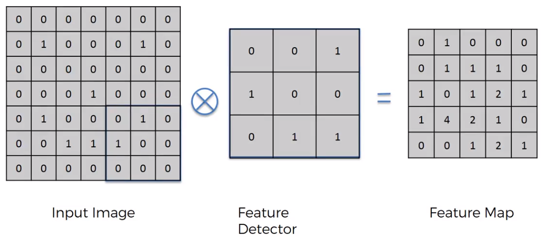
The resulting image on the top right of the figure above is called Feature Map. That essentially is the number of convolved features. The result is a reduction of the input image information. When we have a 2 that means we reduce the image, but a 4 means that we reduce even more the original image, and that make the image easier to be processed. The question is if there are losing information applying the filter Feature Detector. The higher the number we have in the Feature Map, the better is the filtering process and that means we are not losing much feature.
Essentially, we create multiple Feature Maps as many filter of Feature Detection we need (e.g. edge detect, blur detect, emboss detect).
STEP 2 - ReLU Layer This is the Rectified Linear Unit function, an additional step on top of Convolution. The reason why the ReLU is used is to increase the non-linearity. The reason we want to increase non-linearity is because images are highly non-linear, that is why we want to break up linearity.

What the ReLU does for example in a black and white image, is to eliminate the linear component created by the shadows in an image. In fact, shadows are shown in a picture like linear progression of grey scale,and we can exclude using the ReLU this too detailed information.
STEP 3 - Max Pooling Typically, we can have a feature (e.g. a dog) of an image presented in many different positions or orientations. We have to be sure that our neural network has a property called Spatial Invariance. This means, it doesn’t care where the features are located in different environment, or if they are closer, or a bit further apart: our Neural Network need to have the flexibility to find out feature. To obtain that we use Pooling.
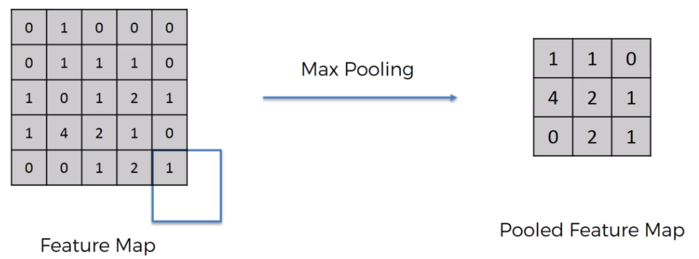
From the figure above, we used the Max Pooling. We take a box of 2x2 pixel from the Feature Map previously created, we find the maximum value, and we report it in the Pooled Feature Map. We repeat this process moving the 2x2 box in the Feature Map. The result is that we are still preserving the features, and because we are taking the maximum of the pixels we are accounting for any distortions and possible spatial or textural or other kind of distortion. Moreover, another benefit of pooling is we are reducing the number of parameters, and so we are preventing overfitting. That is like in humans, because what is important for the vision is not to see exactly all the features that can be noisy, but humans disregarding the unnecessary information. There are lots of types of pooling, and evaluating the type of pooling is crucial. There is a very important article about that which is called: Evaluation of Pooling operations in Convolutional Architectures for Object Recognition by Dominik Scherer. There is also a very useful online tool that we can use to have a better idea about what happen during the Convolution and Pooling process, and we can check the tool by clicking here.
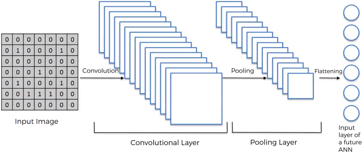
STEP 4 - Flattening The Flattening process simply means to reorder the Pooled Feature Map in a single column. We do that, because this vector now is ready to be used as an input of an ANN for further processing. The entire process describe till now can be summarized by the figure below.
STEP 5 - Full Connection The Flattened vector that we described above, now is used as an input in a Fully Connected ANN. With fully connected we mean that the hidden layer is fully connected. This is by definition a CNN. The purpose of this is to combine our features into more attributes to predict the classes even better. In fact, combining more attributes (e.g. edge detect, blur detect, emboss detect) help to predict better the images. The figure below shows as an example the neurons activated for a Dog.
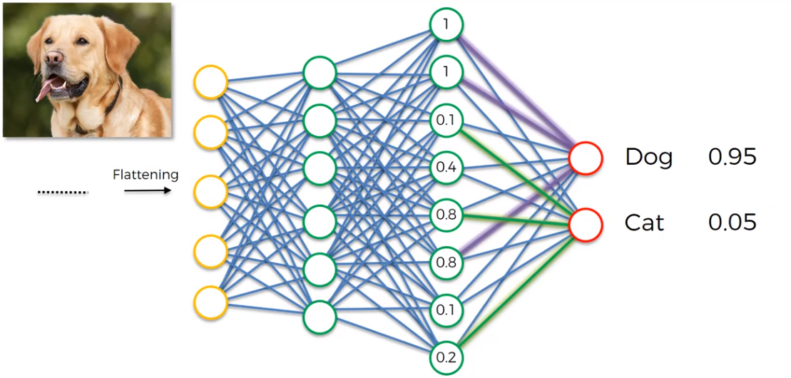
The links between neurons and output colored in violet for dog, and green for cat, tell us which are the important neurons for dog and cat respectively. The figure below, summarize all the steps till now considered.
Softmax and Cross Entropy From the figure about the detection of the dog, we found 0.95 Dog, and 0.05 Cat. The question is how these two values add up to 1. That is possible only introducing the Softmax Function, the formula is the following:
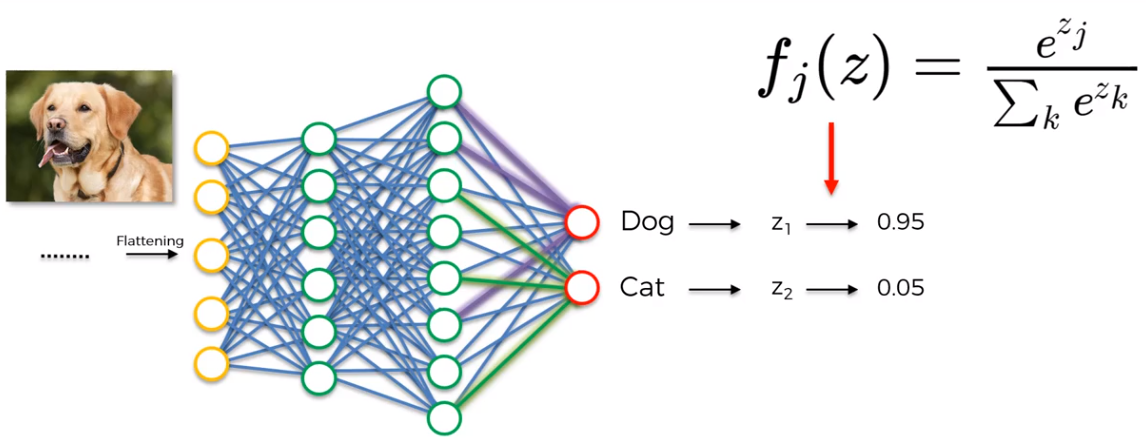
As described by the formula in the figure above, the Softmax Function is a generalization of the Logistic Function, and it makes sure that our prediction add up to 1. Most of the time the Softmax Function is related to the Cross Entropy Function. In CNN, after the application of the Softmax Function, is to test the reliability of the model using as Loss Function the Cross Entropy Function, in order to maximize the performance of our neural network. There are several advantages to using the Cross Entropy Function. One of the best is that if for instance at the start of backpropagation the output value is much smaller than the actual value, the gradient descent will be very slow. Because Cross Entropy uses the logarithm, it helps the network to assess even large errors.
Occipital lobe and CNN It is common to link the Occipital Lobe of the human brain to CNN. In fact, CNNs are responsible for computer vision, recognition of images and objects, which makes them a perfect link to the occipital lobe.