Boltzmann Machine is an Unsupervised Deep Learning used for Recommendation System. Boltzmann Machines are undirected models, they don’t have a direction in the connections as described in the figure below.
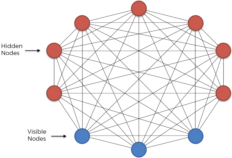
From the figure above, we can see that there is not an output layer. This makes Boltzmann Machine fundamentally different to all other algorithms, and it doesn’t expect input data, but it generates information regardless of input nodes. It is a system. This makes Boltzmann Machine not a deterministic deep learning model but a stochastic deep learning model also called generative deep learning model.
Energy Based Models EBM The equation below is the Boltzmann Distribution.
\[ p_{i}=\frac{e^{-\varepsilon_{i} / k T}}{\sum_{j=1}^{M} e^{-\varepsilon_{j} / k T}} \] Now, image that our system is a nuclear power station. On the left we have the probability of a certain state of our system pi, where i is the state and p the probability of state i. The epsilon is the energy of the system. The k* is a constant and T is the temperature of our system.
The numerator means that the higher the energy of a certain state is, the lower the probability is. So, the probability pi is inversely related to the energy. For example, the gas molecules in a room are uniformly distributed, and the probability to have all the molecules in a corner is low. In fact, in the case the molecules are in the corner the energy is very high. This example explains the equation above.
Restricted Boltzmann Machine RBM It is complicated to implement a complete Boltzmann Machine, because as we increase the number of nodes, the number of connections between them grows exponentially. That is why Restricted Boltzmann Machine RBM is preferred.
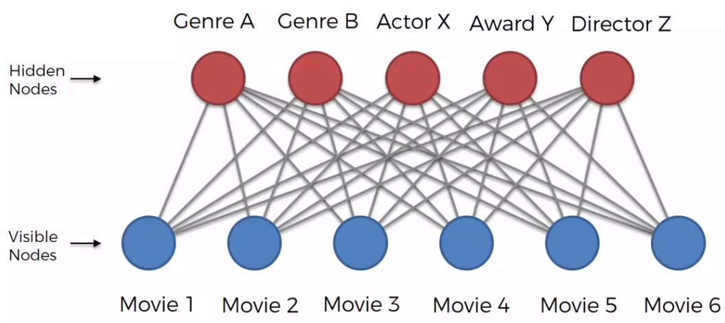
The restriction is that hidden nodes cannot be connected to each other, and visible nodes cannot connect to each other. Other than that, everything is the same. In the example above, we are considering to build a recommender system for movies. RBM is able to auto generate the states of the system, and it is able to identify what kind of features are important to use as recommender. All people have preferences, so, the data we have to deal with are related to the preferences of each person. Now, from the preferences of the movies, we can establish the related features that all movies have in common (e.g. Actor X, Award Y, Direct Z), that make people to like them. This session is called Training Machine on Features.
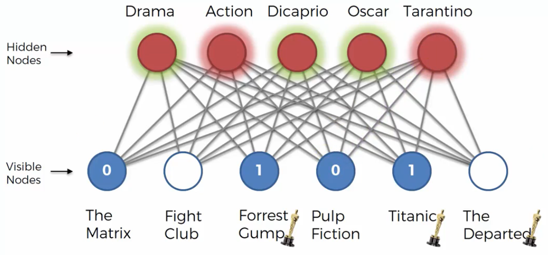
As we can see from the figure above, the hidden nodes are colored in green if the feature is 1=like the movie and in red if the feature is 0=don’t like the movie or empty=movie not seen. Now, RBM tries to reconstruct the empy nodes.
Contrastive Divergence This is the algorithm that allows RBM to learn. It is related to how RBM adjust its weights. In others ANN, we had gradient descent process which allowed us to backpropagate the error through the network, and therefore adjust the weight accordingly. In RBM we don’t have directed network but an undirected network. Now, RBM tries to reconstruct the visible nodes, even the empty nodes. In our example, it reconstruct the movie Fight Club and The Departed, based on what it learned from the training we made before.
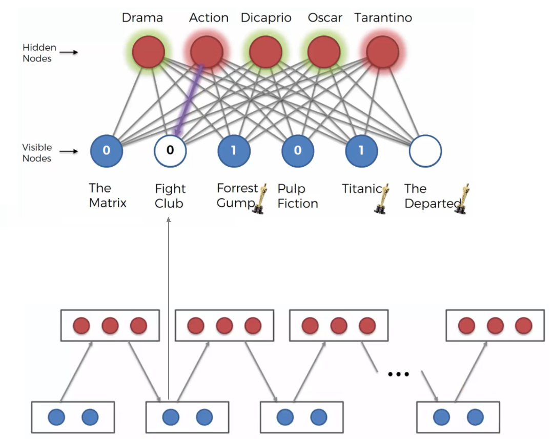
From the figure above, we can see in blue our input nodes, and using arandomly selected weight RBM is able to recognize a hidden node (colored in red in the figure above). After that, the hidden node is able to reconstruct the visible empty node (e.g. the move not seen The Fight Club). This process is called Gibbs Sampling.
Looking at the formula in the figure below, it is a gradient of the log probability of a certain state of our system, based on the weights. The formula says how changing the weights will change the log probability. The visible layer is vi and hidden layer is hi.
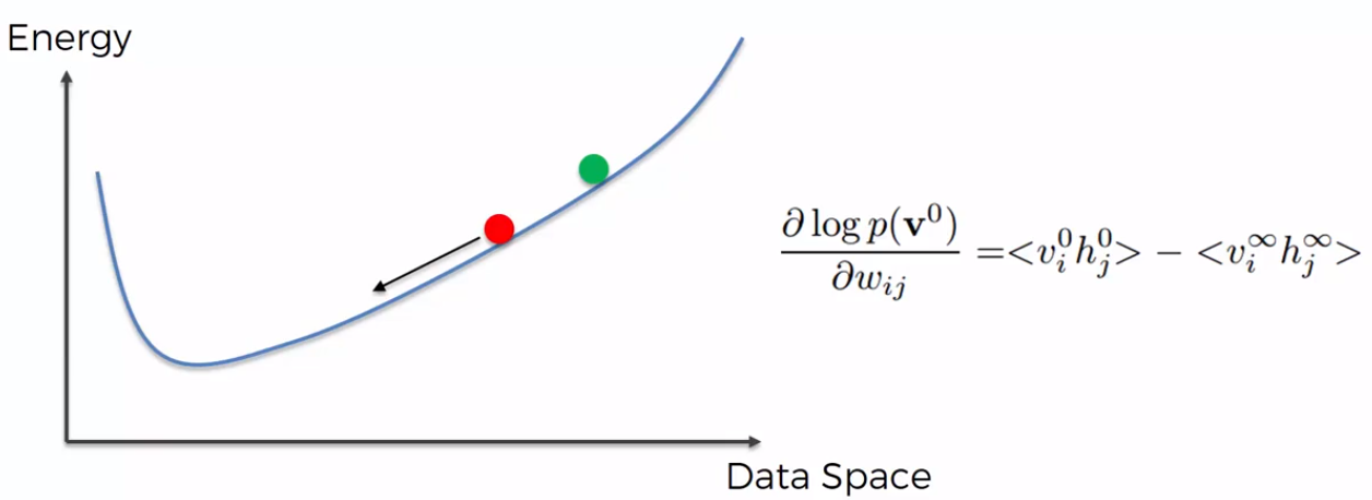
About the Energy Curve depicted on the figure above, we can say that weights dictate the shape of the energy curve. The green circle on the curve is the initial randomly selected weight. The red circle, is generated based on the training, and we try to end up to the lowest energy state possible. Once we arrive to the very lower possible energy, if we subtract the value that we found with the initial randomly selected value, it says to us how adjusting our weights will affect the log probability.
The process till now described is very long, but there is a shortcut: even if we take just the first two steps of the Contrastive Divergence, it is sufficient to understand how to adjust our curve to arrive at the end up (i.e. the lowest energy point). The important thing to keep in mind is the fact that the shape of the Energy Curve is governed by the weights in the system. The Energy Curve reflects the weights and using the subtraction in the formula, we can reach the minimum of the curve very fast. We don’t need to go to the very end of our sampling process.
In its essence, we the Contrastive Divergence tries to adjust the Energy Curve by modifying the weights, in order to facilitate a system in the best way possible. We do that using the formula depicted in the figure above. There is a famous article about this called: A fast learning algorithm for deep belief nets.