This post has the aim to shows all the processes related to the NLP and how to use the Naive Bayes Classifier using Python and the nltk library. We use data from spam detection.
In NLP a large part of the processing is Feature Engeneering. Tipically the steps are: Regular Expression: that is a formal language for specifying text strings: for example, we can have for the same word the s for plural, the capital first letter and any combination of those. We need a methodology to deal with this. Word Tokenization: every language processing has to minimize the text in some way, and we have to start with segmentation also known as tokenization of the words. We have to find the lemma that is same stem or part of the word with the same root. Ones we tokenized our words we need to normalize that words, and also, we have to stem that word in order to reduce inflected words. Moreover, we have to reduce the uppercase in lowercase, with only some exceptions like: General Motors or FED for Federal Reserve Bank, that could be especially helpful in machine translation. Minimum Edit Distance: is the way of solving string similarities. It is ery helpful to correct grammar errors. So, the Minimum Edit Distance between two strings is the minimum number of editing operations (insertion, deletion, substitution) that are needed to transform one string into the other. We often need to use the so called Backtrace Method: similar to DTW to find the minimum distance between two words. Object Standardization: in a text, are often present words or phrases which are not present in a standard lexiconsuch as acronyms, hashtags, colloquial slang. These are very present on social media. We can decide to include them in the stop words list. Bag of words: is used to extract features. We simply count the number of occurrences for each word, this process also called CountVectorizer. To make the CountVectorizer more comparable, we scale it using the Term Frequency Transformation TF, and in order to boost the most important features we use the Inverse Document Frequency IDF, this calculate how often a word occurs in the corpus. The combination of both is called TFiDF = TF * IDF.
\[ \begin{aligned} t f \cdot d t(t, D) &=t f(t, d) \cdot d f(t, D) \\ t f(t, d) &=f_{t \mu} \\ i d f(t, D) &=\log \left(\frac{N}{|\{d \in D: t \in A\}|}\right) \end{aligned} \] TFiDF is the LOG of the total number of documents N divided by the number of documents that contain the term that we are taking into consideration. From the expression above, we have D the toal number of documents, and t number of documents with the term. Matematically we can use the expression reported here below.
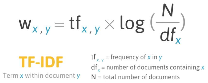
The expression above determ the word Wx in the document y. The formula above give us not only the conut, but also the notation of the importance of a word in the entire corpus of all documents. Now we start with some explortatory data analysis and feature engineering using Python.
messages.groupby('label').describe() # most popular ham and spam messages## message
## count unique top freq
## label
## ham 4825 4516 Sorry, I'll call later 30
## spam 747 653 Please call our customer service representativ... 4messages['length'] = messages['message'].apply(len) # length of the messages
messages.head()## label message length
## 0 ham Go until jurong point, crazy.. Available only ... 111
## 1 ham Ok lar... Joking wif u oni... 29
## 2 spam Free entry in 2 a wkly comp to win FA Cup fina... 155
## 3 ham U dun say so early hor... U c already then say... 49
## 4 ham Nah I don't think he goes to usf, he lives aro... 61messages['length'].describe()## count 5572.000000
## mean 80.489950
## std 59.942907
## min 2.000000
## 25% 36.000000
## 50% 62.000000
## 75% 122.000000
## max 910.000000
## Name: length, dtype: float64From the code above we can see we have a etxt with 910 characters. Here below the text of the message.
messages[messages['length'] == 910]['message'].iloc[0]## "For me the love should start with attraction.i should feel that I need her every time around me.she should be the first thing which comes in my thoughts.I would start the day and end it with her.she should be there every time I dream.love will be then when my every breath has her name.my life should happen around her.my life will be named to her.I would cry for her.will give all my happiness and take all her sorrows.I will be ready to fight with anyone for her.I will be in love when I will be doing the craziest things for her.love will be when I don't have to proove anyone that my girl is the most beautiful lady on the whole planet.I will always be singing praises for her.love will be when I start up making chicken curry and end up makiing sambar.life will be the most beautiful then.will get every morning and thank god for the day because she is with me.I would like to say a lot..will tell later.."There are many methods to convert a corpus of strings to a vector format and the simplest way is usiing bag of words where each unique word in the text will represented by one vector. The first step is to remove punctuation, and stopwords.
import string
from nltk.corpus import stopwords

def text_process(mess):
    """
    Takes in a string of text, then performs the following:
    1. Remove all punctuation
    2. Remove all stopwords
    3. Returns a list of the cleaned text
    """
    # Check characters to see if they are in punctuation
    nopunc = [char for char in mess if char not in string.punctuation]

    # Join the characters again to form the string.
    nopunc = ''.join(nopunc)

    # Now just remove any stopwords
    return [word for word in nopunc.split() if word.lower() not in stopwords.words('english')]

# Check it
messages['message'].head(5).apply(text_process)
## 0    [Go, jurong, point, crazy, Available, bugis, n...
## 1                       [Ok, lar, Joking, wif, u, oni]
## 2    [Free, entry, 2, wkly, comp, win, FA, Cup, fin...
## 3        [U, dun, say, early, hor, U, c, already, say]
## 4    [Nah, dont, think, goes, usf, lives, around, t...
## Name: message, dtype: object
Now, we can focus on vectorization namely count how many times a word occur in a text, and this is called Term Frequency. We have also to normalize the vector to unit length. Since there are so many messages, we can expect lot of zeros. Because of this, we can use SciKit Learn to otput a Sparse Matrix.
from sklearn.feature_extraction.text import CountVectorizer

# Create bag of words
bow_transformer = CountVectorizer(analyzer=text_process).fit(messages['message'])

# Check the sparsity
messages_bow = bow_transformer.transform(messages['message'])
print('Shape of Sparse Matrix: ', messages_bow.shape)
## Shape of Sparse Matrix: (5572, 11425)print('Amount of Non-Zero occurences: ', messages_bow.nnz)## Amount of Non-Zero occurences: 50548sparsity = (100.0 * messages_bow.nnz / (messages_bow.shape[0] * messages_bow.shape[1]))
print('sparsity: {}'.format(sparsity))## sparsity: 0.07940295412668218Now that we have an idea about the sparsity of of bag of word, we can calculate the TF-IDF. TF: Term Frequency, which measures how frequently a term occurs in a document. Since every document is different in length, it is possible that a term would appear much more times in long documents than shorter ones. Thus, the term frequency is often divided by the document length (aka. the total number of terms in the document) as a way of normalization: TF(t) = (Number of times term t appears in a document) / (Total number of terms in the document).
IDF: Inverse Document Frequency, which measures how important a term is. While computing TF, all terms are considered equally important. However it is known that certain terms, such as “is”, “of”, and “that”, may appear a lot of times but have little importance. Thus we need to weigh down the frequent terms while scale up the rare ones, by computing the following: IDF(t) = log_e(Total number of documents / Number of documents with term t in it).
from sklearn.feature_extraction.text import TfidfTransformer

tfidf_transformer = TfidfTransformer().fit(messages_bow) # inverse document frequency and term relationship frequency
print(tfidf_transformer.idf_[bow_transformer.vocabulary_['u']]) # check the imprtance of u
## 3.2800524267409408print(tfidf_transformer.idf_[bow_transformer.vocabulary_['university']]) # check the imprtance of the word university
## 8.527076498901426Now we are ready to create the classifier model. Naive Bayes is a good baseline for text classification. In sentiment analysis, for example the target can be positive or negative. Naive Bayes is based on conditional independence assumption.
\[ P\left(d o c | v_{j}\right)=\prod_{i=1}^{l e n g t h(d o c)} P\left(a_{i}=w_{k} | v_{j}\right) \]
Now, the probability of a document belonging to a certain class (let’s say positive) is: the length of the doc, multiplied to the probability that each word is classified as positive. The probability of a word given a positive outcome is the number of times the word k is present in positive cases divided by the total number of words of positive cases, plus the size of the vocabulary. We can classify the sentence based on the formula here below.
\[ V_{N B}=\underset{v \in V}{\operatorname{argmax}} P\left(v_{j}\right) \prod_{w \in \text { words }} P\left(w | v_{j}\right) \]
The value of the Naive Bayes VBN is the value that gives me the highest number argmax when I compute the probability of each of the words given the positive case. The arguments of the maxima arg are the points, or elements, of the domain of some function at which the function values are maximized. We perform the Naive Bayes model using the pipeline function of Python that semplify the steps till now described.
from sklearn.naive_bayes import MultinomialNB
from sklearn.pipeline import Pipeline

pipeline = Pipeline([
    ('bow', CountVectorizer(analyzer=text_process)),  # strings to token integer counts
    ('tfidf', TfidfTransformer()),  # integer counts to weighted TF-IDF scores
    ('classifier', MultinomialNB()),  # train on TF-IDF vectors w/ Naive Bayes classifier
])

# Split the data in Test and Train and make Prediction
from sklearn.model_selection import train_test_split
msg_train, msg_test, label_train, label_test = train_test_split(messages['message'], messages['label'], test_size=0.2)
pipeline.fit(msg_train,label_train)
## Pipeline(memory=None,
## steps=[('bow', CountVectorizer(analyzer=<function text_process at 0x000000002B2A4158>,
## binary=False, decode_error='strict', dtype=<class 'numpy.int64'>,
## encoding='utf-8', input='content', lowercase=True, max_df=1.0,
## max_features=None, min_df=1, ngram_range=(1, 1), preprocesso...f=False, use_idf=True)), ('classifier', MultinomialNB(alpha=1.0, class_prior=None, fit_prior=True))])predictions = pipeline.predict(msg_test)
# Elavuate the Model
from sklearn.metrics import classification_report
print(classification_report(predictions,label_test))## precision recall f1-score support
##
## ham 1.00 0.96 0.98 1004
## spam 0.74 1.00 0.85 111
##
## micro avg 0.96 0.96 0.96 1115
## macro avg 0.87 0.98 0.91 1115
## weighted avg 0.97 0.96 0.97 1115We found a 96% of precision which is retty good considering that we are dealing with text data. To have a better undersanding about the Model Evaluation the figure below it is a good description of the metrics we are using.
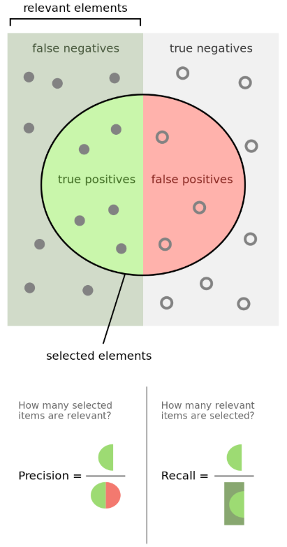
There are quite a few possible metrics for evaluating model performance. Which one is the most important depends on the task and the business effects of decisions based off of the model. For example, the cost of mis-predicting “spam” as “ham” is probably much lower than mis-predicting “ham” as “spam”.