Extreme Gradient Boosting is extensively used because is fast and accurate, and can handle missing values. Gradient boosting is a machine learning technique for regression and classification problems, which produces a prediction model in the form of an ensemble of weak prediction models, typically decision trees. It builds the model in a stage-wise fashion like other boosting methods do, and it generalizes them by allowing optimization of an arbitrary differentiable loss function. XGBoost is one of the implementations of Gradient Boosting concept, but what makes XGBoost unique is that it uses a more regularized model formalization to control over-fitting, which gives it better performance.
We use it in an example to predict, based on some features (e.g. the rank of the school student come from), if a student is admitted or rejected.
# Partition Data
set.seed(1234)
ind <- sample(2, nrow(data), replace = T, prob = c(0.8, 0.2))
train <- data[ind==1,]
test <- data[ind==2,]

# Create matrix One-Hot Encoding for Factor variables.
# One-Hot Encoding convert our data in a numeric format, as required by XGBoost.
# It convert the variable rank in a sparse matrix, in order to have dummy variable for each rank.
trainm <- sparse.model.matrix(admit ~ .-1, data = train)
head(trainm)
6 x 6 sparse Matrix of class "dgCMatrix"
gre gpa rank1 rank2 rank3 rank4
1 380 3.61 . . 1 .
2 660 3.67 . . 1 .
3 800 4.00 1 . . .
4 640 3.19 . . . 1
6 760 3.00 . 1 . .
7 560 2.98 1 . . .# Convert Train-Set in a Matrix
train_label <- train[,"admit"] # define the responce variable
train_matrix <- xgb.DMatrix(data = as.matrix(trainm), label = train_label)From the matrix above, we can see that One-Hot Encoding was made for the factor variabile (i.e. rank). We repeat the same procedure for the Test-set.
# Convert Test-Set in a Matrix
testm <- sparse.model.matrix(admit ~ .-1, data = test)
test_label <- test[,"admit"] # define the responce variable
test_matrix <- xgb.DMatrix(data = as.matrix(testm), label = test_label)
For now, we have the matrix formatted in the proper format needed for the analysis. At this stage, we have to define the parameters of the model, and create it.
nc <- length(unique(train_label))
xgb_params <- list("objective" = "multi:softprob",
                   "eval_metric" = "mlogloss",
                   "num_class" = nc)

watchlist <- list(train = train_matrix, test = test_matrix)

# Create the Extreme Gradient Boosting Model
bst_model <- xgb.train(params = xgb_params,    # multiclass classification
                       data = train_matrix,
                       nrounds = 20,           # maximum number of interations
                       watchlist = watchlist)  # check what is going on
[1] train-mlogloss:0.594324 test-mlogloss:0.651085
[2] train-mlogloss:0.534790 test-mlogloss:0.612848
[3] train-mlogloss:0.483394 test-mlogloss:0.595096
[4] train-mlogloss:0.454567 test-mlogloss:0.597930
[5] train-mlogloss:0.423043 test-mlogloss:0.599238
[6] train-mlogloss:0.385208 test-mlogloss:0.595708
[7] train-mlogloss:0.372651 test-mlogloss:0.614298
[8] train-mlogloss:0.355396 test-mlogloss:0.612562
[9] train-mlogloss:0.345466 test-mlogloss:0.632218
[10] train-mlogloss:0.337584 test-mlogloss:0.649025
[11] train-mlogloss:0.321141 test-mlogloss:0.649074
[12] train-mlogloss:0.312773 test-mlogloss:0.664441
[13] train-mlogloss:0.309723 test-mlogloss:0.677517
[14] train-mlogloss:0.296634 test-mlogloss:0.677277
[15] train-mlogloss:0.284527 test-mlogloss:0.689391
[16] train-mlogloss:0.277117 test-mlogloss:0.684779
[17] train-mlogloss:0.270126 test-mlogloss:0.688089
[18] train-mlogloss:0.265546 test-mlogloss:0.701466
[19] train-mlogloss:0.260600 test-mlogloss:0.700825
[20] train-mlogloss:0.256453 test-mlogloss:0.717978 bst_model##### xgb.Booster
raw: 69.1 Kb
call:
xgb.train(params = xgb_params, data = train_matrix, nrounds = 20,
watchlist = watchlist)
params (as set within xgb.train):
objective = "multi:softprob", eval_metric = "mlogloss", num_class = "2", silent = "1"
xgb.attributes:
niter
callbacks:
cb.print.evaluation(period = print_every_n)
cb.evaluation.log()
# of features: 6
niter: 20
nfeatures : 6
evaluation_log:
iter train_mlogloss test_mlogloss
1 0.594324 0.651085
2 0.534790 0.612848
---
19 0.260600 0.700825
20 0.256453 0.717978In the code above we specified to use the Softprob Function. In Softmax we get the class with the maximum probability as output, and with Softprob we get a matrix with probability value of each class we are trying to predict. We can also see that we have as output the total number of interations (in our example 20 interactions), and we can see what was the error in both train and test set (aka elaluation_log). We have also some information about the model. The elaluation_log session of the output can be converted into a plot.
# Training and Test Error Plot
e <- data.frame(bst_model$evaluation_log)
plot(e$iter, e$train_mlogloss, col = 'blue')
lines(e$iter, e$test_mlogloss, col = 'red')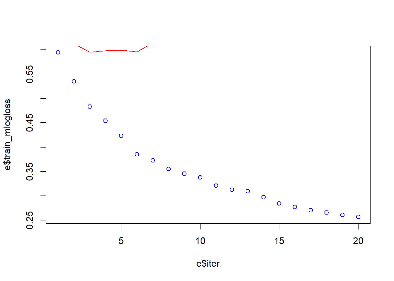
min(e$test_mlogloss)[1] 0.595096e[e$test_mlogloss == 0.595096,] iter train_mlogloss test_mlogloss
3 3 0.483394 0.595096We can see from the graph above that the error, in the Training-set, is quite high in the beginning and as the interactions increase the error comes down. The little curve in red that we have on the top right of the graph is the error rate of the Test-set: initially the error quickly comes down but immediately increases. We can see that we have a Minimum Error of the Test-set of 0.59 at we reach it after 3 interations. This red curve says that we have a significat overfitting. We need to find a better model.
# More feature to find the best model
bst_model <- xgb.train(params = xgb_params,    # multiclass classification
                       data = train_matrix,
                       nrounds = 20,           # maximum number of interations
                       watchlist = watchlist,
                       eta = 0.05)             # is eta is low, the model is more robust to overfitting
[1] train-mlogloss:0.674595 test-mlogloss:0.684052
[2] train-mlogloss:0.658466 test-mlogloss:0.676982
[3] train-mlogloss:0.642685 test-mlogloss:0.667532
[4] train-mlogloss:0.628284 test-mlogloss:0.660133
[5] train-mlogloss:0.615050 test-mlogloss:0.653341
[6] train-mlogloss:0.604056 test-mlogloss:0.645568
[7] train-mlogloss:0.592582 test-mlogloss:0.640064
[8] train-mlogloss:0.582170 test-mlogloss:0.637070
[9] train-mlogloss:0.571289 test-mlogloss:0.634656
[10] train-mlogloss:0.561741 test-mlogloss:0.630252
[11] train-mlogloss:0.551731 test-mlogloss:0.628331
[12] train-mlogloss:0.542504 test-mlogloss:0.622866
[13] train-mlogloss:0.533755 test-mlogloss:0.618194
[14] train-mlogloss:0.525246 test-mlogloss:0.617723
[15] train-mlogloss:0.517447 test-mlogloss:0.613506
[16] train-mlogloss:0.509825 test-mlogloss:0.613574
[17] train-mlogloss:0.502859 test-mlogloss:0.609476
[18] train-mlogloss:0.496269 test-mlogloss:0.606218
[19] train-mlogloss:0.489355 test-mlogloss:0.606840
[20] train-mlogloss:0.483546 test-mlogloss:0.604335 e <- data.frame(bst_model$evaluation_log)
plot(e$iter, e$train_mlogloss, col = 'blue')
lines(e$iter, e$test_mlogloss, col = 'red')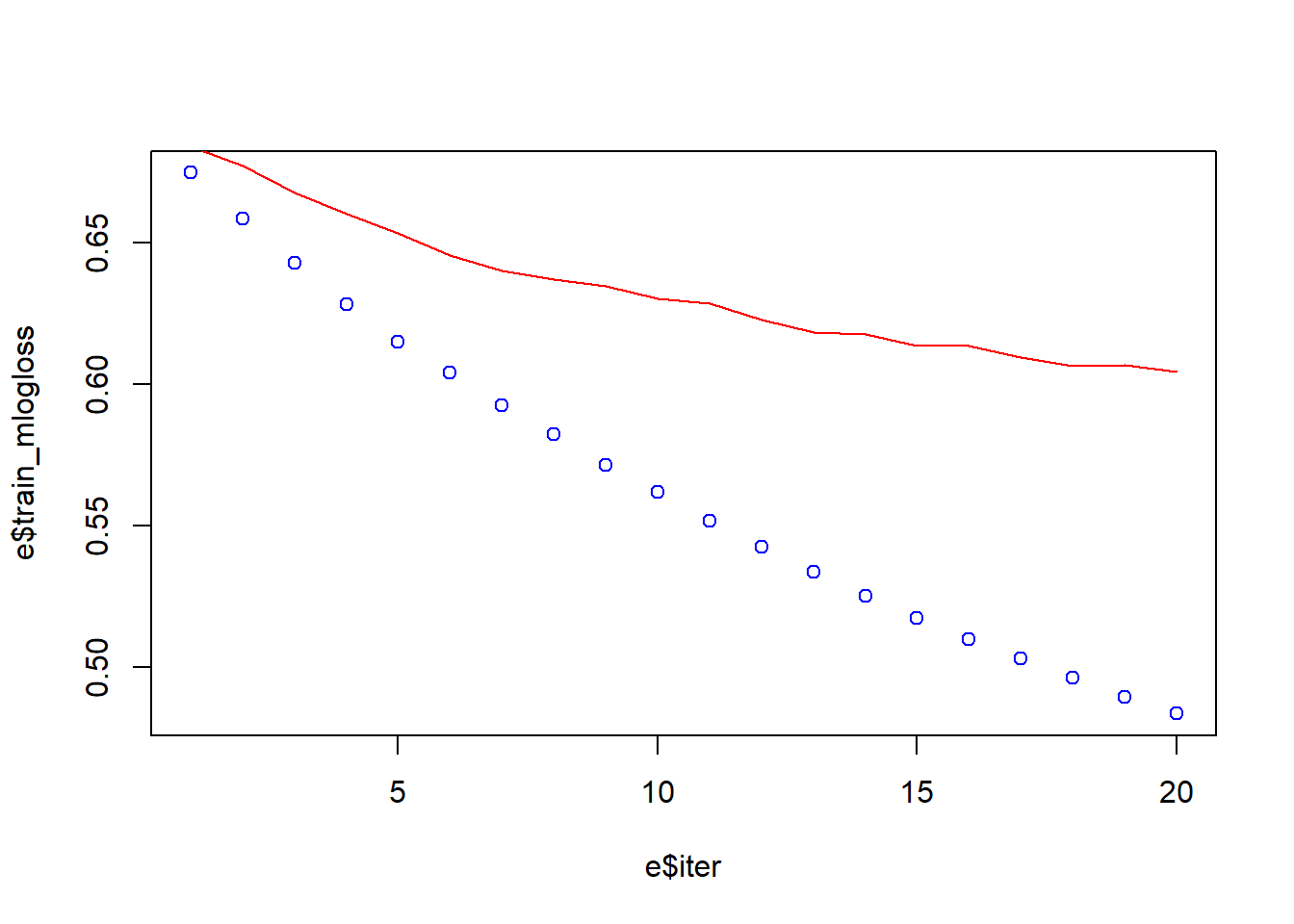
Now, that we have introduce the learning rate Eta the performance is better. The range of Eta is between 0 and 1, we use eta = 0.05 because with low eta the model is more robust to overfitting. The Eta Learning Rate is the shrinkage you do at every step you are making. If you make 1 step at eta = 1.00, the step weight is 1.00. If you make 1 step at eta = 0.25, the step weight is 0.25. If our learning rate is 1.00, we will either land on 5 or 6 (in either 5 or 6 computation steps) which is not the optimum we are looking for. If our learning rate is 0.10, we will either land on 5.2 or 5.3 (in either 52 or 53 computation steps), which is better than the previous optimum. If our learning rate is 0.01, we will either land on 5.23 or 5.24 (in either 523 or 534 computation steps), which is again better than the previous optimum. At this stage, we can introduce the Feature Importanc information.
# Feature Importance
imp <- xgb.importance(colnames(train_matrix), model = bst_model)
print(imp)
Feature Gain Cover Frequency
1: gpa 0.54922337 0.496645022 0.45471349
2: gre 0.28520228 0.315538132 0.39556377
3: rank1 0.11819828 0.099514082 0.05360444
4: rank2 0.02775006 0.081352562 0.06284658
5: rank4 0.01962602 0.006950201 0.03327172xgb.plot.importance(imp)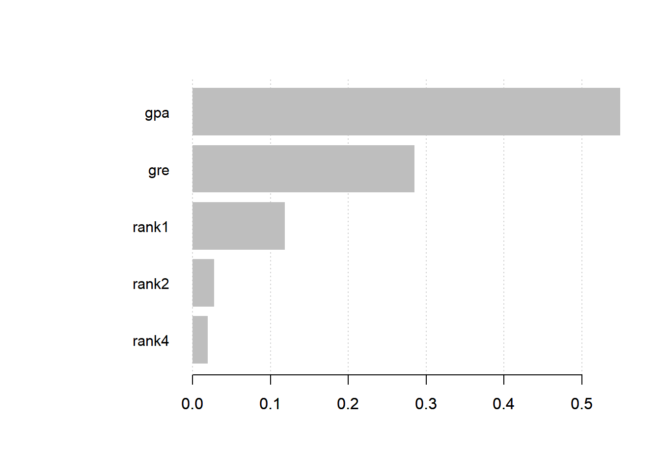
From the table above, Gain is the most important column. It says to us that the variable gpa has the most importance. We have the same result graphically (the graph is made using Gain as parameter).
We can do prediction and create confusion matrix using thet Test-set.
# Prediction and Confusion Matrix on Test-set
p <- predict(bst_model, newdata = test_matrix) # calculate prediction
pred <- matrix(p, nrow = nc, ncol = length(p)/nc) %>%
         t() %>%           # transpose the matrix
         data.frame() %>%  # transform in a data frame
         mutate(label = test_label, max_prob = max.col(., "last")-1) #

head(pred)
X1 X2 label max_prob
1 0.7922649 0.2077352 0 0
2 0.6508374 0.3491626 0 0
3 0.6971229 0.3028770 0 0
4 0.3676542 0.6323458 1 1
5 0.4761441 0.5238559 1 1
6 0.4498452 0.5501549 1 1# Confusion Matrix
table(Prediction = pred$max_prob, Actual = pred$label) Actual
Prediction 0 1
0 43 19
1 7 6What we can see from the table above, is X1 (the probability to be not admitted), X2 (the probability to be admitted). The label is the actual label in the Test-set (i.e. the real values), the max_prob is the label predicted. If we look at the row number 5 we see a proability to be not admitted (X1=0.51, max_prob=0), but the reality is that student was admitted (label=1). If we look at the Confusion Matrix, we have an Accuracy of (43+7)75=66%, and so we can try again to improve the model.
# More XGBoost Parameters
bst_model <- xgb.train(params = xgb_params,    # multiclass classification
                       data = train_matrix,
                       nrounds = 20,           # maximum number of interations
                       watchlist = watchlist,
                       eta = 0.01,             # is eta is low, the model is more robust to overfitting
                       max.depth = 3,          # maximum tree depth
                       gamma = 0,              # larger values of gamma lead to more conservative algorithm
                       subsample = 1,          # 1 means 100%, lower values help to prevent overfitting
                       colsample_bytre = 1,
                       missing = NA,
                       seed = 333)
[1] train-mlogloss:0.690576 test-mlogloss:0.691426
[2] train-mlogloss:0.688062 test-mlogloss:0.689451
[3] train-mlogloss:0.685597 test-mlogloss:0.687521
[4] train-mlogloss:0.683178 test-mlogloss:0.685633
[5] train-mlogloss:0.680805 test-mlogloss:0.683788
[6] train-mlogloss:0.678476 test-mlogloss:0.681985
[7] train-mlogloss:0.676192 test-mlogloss:0.680221
[8] train-mlogloss:0.673950 test-mlogloss:0.678497
[9] train-mlogloss:0.671750 test-mlogloss:0.676812
[10] train-mlogloss:0.669590 test-mlogloss:0.675196
[11] train-mlogloss:0.667471 test-mlogloss:0.673466
[12] train-mlogloss:0.665389 test-mlogloss:0.671922
[13] train-mlogloss:0.663345 test-mlogloss:0.670264
[14] train-mlogloss:0.661337 test-mlogloss:0.668787
[15] train-mlogloss:0.659366 test-mlogloss:0.667199
[16] train-mlogloss:0.657430 test-mlogloss:0.665788
[17] train-mlogloss:0.655528 test-mlogloss:0.664264
[18] train-mlogloss:0.653661 test-mlogloss:0.662893
[19] train-mlogloss:0.651826 test-mlogloss:0.661433
[20] train-mlogloss:0.650024 test-mlogloss:0.660144 e <- data.frame(bst_model$evaluation_log)
plot(e$iter, e$train_mlogloss, col = 'blue')
lines(e$iter, e$test_mlogloss, col = 'red')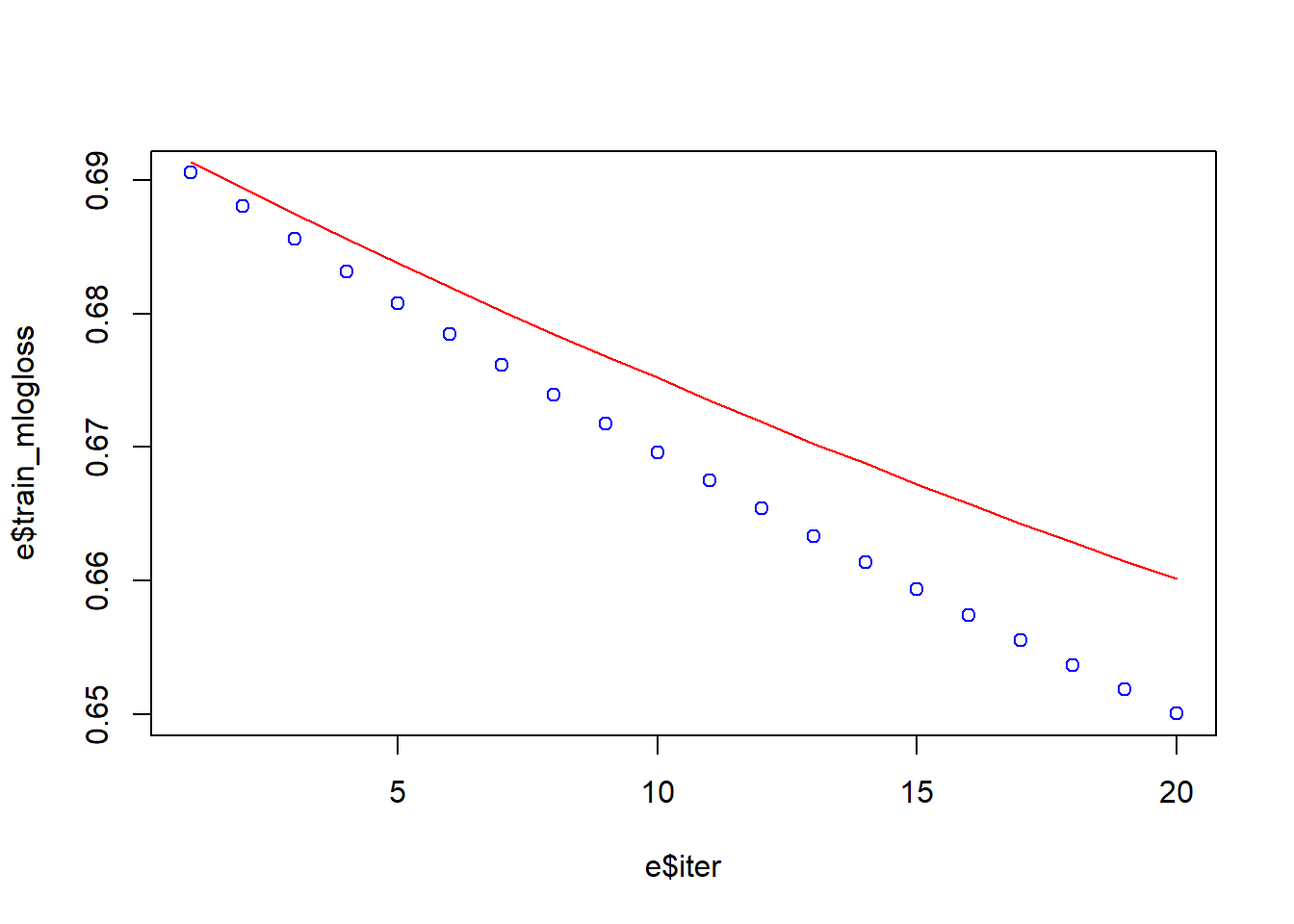
It the model descrbed above, we introduced five new parameters.
The max_depth indicates how deep the tree can be. The deeper the tree, the more splits it has and it captures more information about the data. The gamma mathematically is the Lagrangian Multiplier, which is a method to find the local maxima and minima of a function. We can start to increase gamma value gradually in order to avoid overfitting at look at the graph the result. The parameter missing help to handle with missing values. The seed assure that we can repeat the result.
What we can see now from the graph, we were able to reduce the overfitting.