This is a regression technique that can helps us alleviate the problem of outliers. Robust Regression is a family of regression techniques that is really quite immune to the presence of outliers. Least Trimmed Squares Regression is a technique that fit a regression function and is not effected by the presence of outliers. Least Trimmed Squares Regression attempts to minimise the sum of squared residuals over a subset of k points.
library(mlbench)
library(robustbase)
data(BostonHousing)
str(BostonHousing)
'data.frame': 506 obs. of 14 variables:
$ crim : num 0.00632 0.02731 0.02729 0.03237 0.06905 ...
$ zn : num 18 0 0 0 0 0 12.5 12.5 12.5 12.5 ...
$ indus : num 2.31 7.07 7.07 2.18 2.18 2.18 7.87 7.87 7.87 7.87 ...
$ chas : Factor w/ 2 levels "0","1": 1 1 1 1 1 1 1 1 1 1 ...
$ nox : num 0.538 0.469 0.469 0.458 0.458 0.458 0.524 0.524 0.524 0.524 ...
$ rm : num 6.58 6.42 7.18 7 7.15 ...
$ age : num 65.2 78.9 61.1 45.8 54.2 58.7 66.6 96.1 100 85.9 ...
$ dis : num 4.09 4.97 4.97 6.06 6.06 ...
$ rad : num 1 2 2 3 3 3 5 5 5 5 ...
$ tax : num 296 242 242 222 222 222 311 311 311 311 ...
$ ptratio: num 15.3 17.8 17.8 18.7 18.7 18.7 15.2 15.2 15.2 15.2 ...
$ b : num 397 397 393 395 397 ...
$ lstat : num 4.98 9.14 4.03 2.94 5.33 ...
$ medv : num 24 21.6 34.7 33.4 36.2 28.7 22.9 27.1 16.5 18.9 ...reg1 <- lm(medv ~., data =BostonHousing)
summary(reg1)
Call:
lm(formula = medv ~ ., data = BostonHousing)

Residuals:
    Min      1Q  Median      3Q     Max
-15.595  -2.730  -0.518   1.777  26.199

Coefficients:
              Estimate Std. Error t value Pr(>|t|)
(Intercept)  3.646e+01  5.103e+00   7.144 3.28e-12 ***
crim        -1.080e-01  3.286e-02  -3.287 0.001087 **
zn           4.642e-02  1.373e-02   3.382 0.000778 ***
indus        2.056e-02  6.150e-02   0.334 0.738288
chas1        2.687e+00  8.616e-01   3.118 0.001925 **
nox         -1.777e+01  3.820e+00  -4.651 4.25e-06 ***
rm           3.810e+00  4.179e-01   9.116  < 2e-16 ***
age          6.922e-04  1.321e-02   0.052 0.958229
dis         -1.476e+00  1.995e-01  -7.398 6.01e-13 ***
rad          3.060e-01  6.635e-02   4.613 5.07e-06 ***
tax         -1.233e-02  3.760e-03  -3.280 0.001112 **
ptratio     -9.527e-01  1.308e-01  -7.283 1.31e-12 ***
b            9.312e-03  2.686e-03   3.467 0.000573 ***
lstat       -5.248e-01  5.072e-02 -10.347  < 2e-16 ***
---
Signif. codes:  0 '***' 0.001 '**' 0.01 '*' 0.05 '.' 0.1 ' ' 1

Residual standard error: 4.745 on 492 degrees of freedom
Multiple R-squared:  0.7406,    Adjusted R-squared:  0.7338
F-statistic: 108.1 on 13 and 492 DF,  p-value: < 2.2e-16
plot(reg1)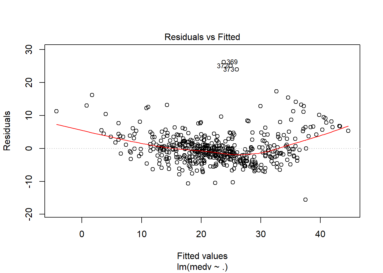
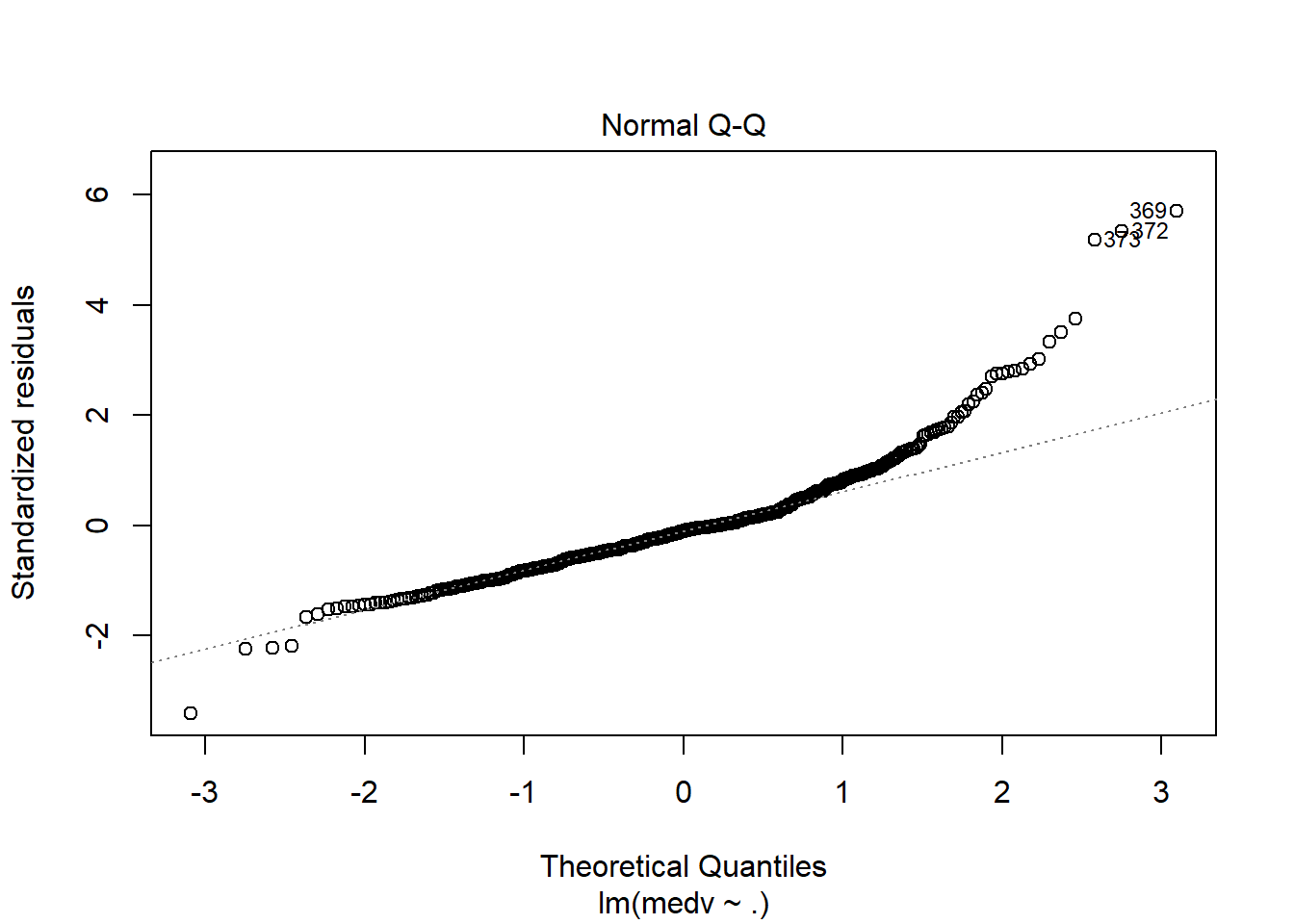
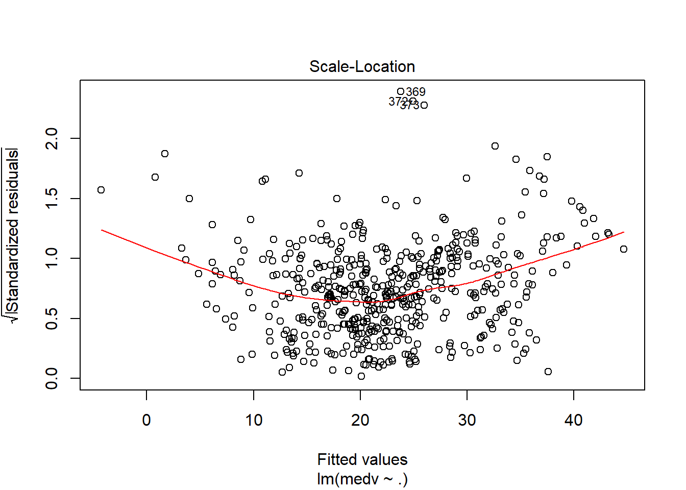
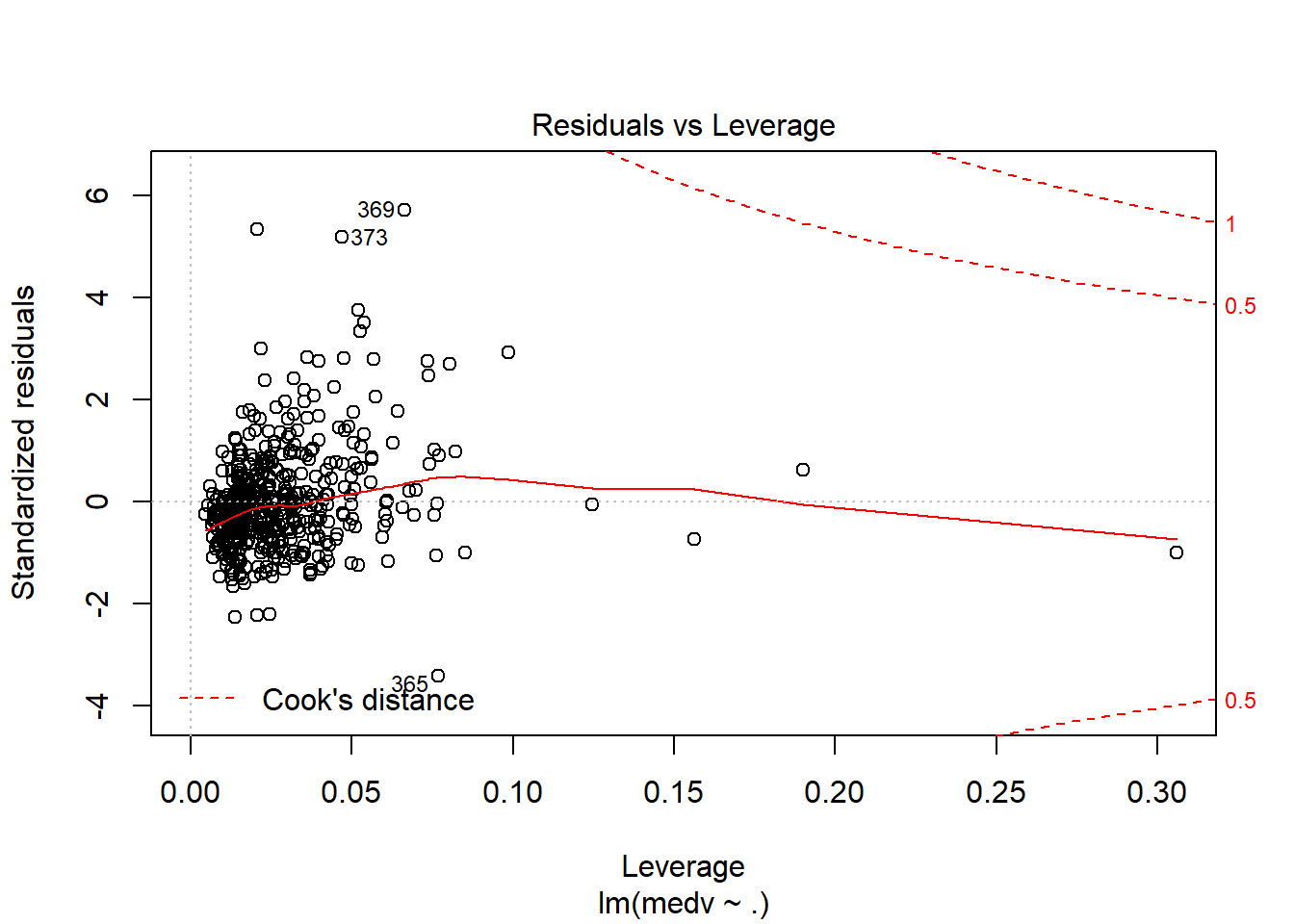
As we can see from the results above, most of the predictor are statistically significant. The Adjsted R-squared values is 0.73, and the p-value is less than 0.05 which make the model statistically significant. The model explain the 73% of variation of the response variable. Looking at the last graph resuduals vs. leverage, it sayas to us that observations 369 and 373 are outliers. We can also test is and run a Robust Regression.
library(car)
outlierTest(reg1) #identify the outlier data pts
rstudent unadjusted p-value Bonferonni p
369 5.907411 6.4998e-09 3.2889e-06
372 5.491079 6.4185e-08 3.2478e-05
373 5.322247 1.5617e-07 7.9020e-05library(robustbase)
ltsFit = ltsReg(medv ~., data =BostonHousing)
summary(ltsFit)
Call:
ltsReg.formula(formula = medv ~ ., data = BostonHousing)

Residuals (from reweighted LS):
   Min     1Q Median     3Q    Max
-7.047 -1.340  0.000  1.306  7.086

Coefficients:
           Estimate Std. Error t value Pr(>|t|)
Intercept  7.133193   3.586372   1.989  0.04733 *
crim      -0.507579   0.053559  -9.477  < 2e-16 ***
zn         0.033001   0.008588   3.843  0.00014 ***
indus     -0.002682   0.036204  -0.074  0.94099
chas1      1.175452   0.548071   2.145  0.03253 *
nox       -3.064635   2.274219  -1.348  0.17850
rm         5.457775   0.346509  15.751  < 2e-16 ***
age       -0.054621   0.008078  -6.762 4.41e-11 ***
dis       -0.912505   0.122830  -7.429 5.86e-13 ***
rad        0.222938   0.042951   5.191 3.23e-07 ***
tax       -0.009213   0.002152  -4.281 2.29e-05 ***
ptratio   -0.556512   0.077393  -7.191 2.84e-12 ***
b          0.010373   0.001665   6.230 1.10e-09 ***
lstat     -0.162327   0.036601  -4.435 1.17e-05 ***
---
Signif. codes:  0 '***' 0.001 '**' 0.01 '*' 0.05 '.' 0.1 ' ' 1

Residual standard error: 2.667 on 434 degrees of freedom
Multiple R-Squared: 0.8442, Adjusted R-squared: 0.8396
F-statistic: 180.9 on 13 and 434 DF,  p-value: < 2.2e-16
The key thing that we can see from the result above is that the Adjusted R-Squared value is grown up to 0.82, now 83% of the variation of the response variable is expained ny predictors.